ファイルサーバ兼深層学習プラットフォームとして使用するつもりでTX1310M3を入手してみた。
これまで富士通のサーバにはCentOS7をインストールして使ってきたのだが、深層学習プラットフォームとしてはRedhat系のCentOSよりDebian系のUbuntuの方が構築しやすいことがわかっていたのでUbuntuをインストールしたいのだが、富士通とUbuntuはあんまり相性が良くないのかもしれない。
というのもTX1310M3が備えているembedded software RAIDはRedHat系でしかドライバが供給されていないので使えない。かといってUbuntuはCentOS7よりRAIDの対応がイマイチでOS組み込みのsoftware RAIDをOSのインストーラで簡単に設定できるようにはなっていないようだ。さてどうしたものか。
ヤフオクで2000円で入手したNECのExpress 5800 T110f-Eの方はhardware RAIDカードを持っているのでRAID上にUbuntuのインストールも簡単に行えた。
うーん、TX1310M3をファイルサーバにするならUbuntuではなくCentOS7にするべきだし、深層学習するなら起動ディスクはRAIDを組まずにUbuntuを入れるべきだ、ということでやはりどちらも専用で用意するしかないね。ファイルサーバはこれまで使ってきたExpress5800R110eの方に任せることにしてTX1310M3は深層学習専用とすることにしよう。
T110f-EはRAIDとUbuntuが両立出来ているのでいいのだが、pci eスロットの制約があって結局RAIDとビデオカードが両立できないという難しさ。やはり既製のサーバではなくカスタムメイドで専用機を建てるようにすべきなんだろうな。
deeplearning テキストの2値化
:~$ python3
Python 3.6.9 (default, Nov  7 2019, 10:44:02)
[GCC 8.3.0] on linux
Type "help", "copyright", "credits" or "license" for more information.
>>> from keras.datasets import imdb
/usr/lib/python3/dist-packages/h5py/__init__.py:36: FutureWarning: Conversion of the second argument of issubdtype from `float` to `np.floating` is deprecated. In future, it will be treated as `np.float64 == np.dtype(float).type`.
  from ._conv import register_converters as _register_converters
Using TensorFlow backend.
/usr/local/lib/python3.6/dist-packages/tensorflow/python/framework/dtypes.py:516: FutureWarning: Passing (type, 1) or '1type' as a synonym of type is deprecated; in a future version of numpy, it will be understood as (type, (1,)) / '(1,)type'.
  _np_qint8 = np.dtype([("qint8", np.int8, 1)])
/usr/local/lib/python3.6/dist-packages/tensorflow/python/framework/dtypes.py:517: FutureWarning: Passing (type, 1) or '1type' as a synonym of type is deprecated; in a future version of numpy, it will be understood as (type, (1,)) / '(1,)type'.
  _np_quint8 = np.dtype([("quint8", np.uint8, 1)])
/usr/local/lib/python3.6/dist-packages/tensorflow/python/framework/dtypes.py:518: FutureWarning: Passing (type, 1) or '1type' as a synonym of type is deprecated; in a future version of numpy, it will be understood as (type, (1,)) / '(1,)type'.
  _np_qint16 = np.dtype([("qint16", np.int16, 1)])
/usr/local/lib/python3.6/dist-packages/tensorflow/python/framework/dtypes.py:519: FutureWarning: Passing (type, 1) or '1type' as a synonym of type is deprecated; in a future version of numpy, it will be understood as (type, (1,)) / '(1,)type'.
  _np_quint16 = np.dtype([("quint16", np.uint16, 1)])
/usr/local/lib/python3.6/dist-packages/tensorflow/python/framework/dtypes.py:520: FutureWarning: Passing (type, 1) or '1type' as a synonym of type is deprecated; in a future version of numpy, it will be understood as (type, (1,)) / '(1,)type'.
  _np_qint32 = np.dtype([("qint32", np.int32, 1)])
/usr/local/lib/python3.6/dist-packages/tensorflow/python/framework/dtypes.py:525: FutureWarning: Passing (type, 1) or '1type' as a synonym of type is deprecated; in a future version of numpy, it will be understood as (type, (1,)) / '(1,)type'.
  np_resource = np.dtype([("resource", np.ubyte, 1)])
/usr/local/lib/python3.6/dist-packages/tensorboard/compat/tensorflow_stub/dtypes.py:541: FutureWarning: Passing (type, 1) or '1type' as a synonym of type is deprecated; in a future version of numpy, it will be understood as (type, (1,)) / '(1,)type'.
  _np_qint8 = np.dtype([("qint8", np.int8, 1)])
/usr/local/lib/python3.6/dist-packages/tensorboard/compat/tensorflow_stub/dtypes.py:542: FutureWarning: Passing (type, 1) or '1type' as a synonym of type is deprecated; in a future version of numpy, it will be understood as (type, (1,)) / '(1,)type'.
  _np_quint8 = np.dtype([("quint8", np.uint8, 1)])
/usr/local/lib/python3.6/dist-packages/tensorboard/compat/tensorflow_stub/dtypes.py:543: FutureWarning: Passing (type, 1) or '1type' as a synonym of type is deprecated; in a future version of numpy, it will be understood as (type, (1,)) / '(1,)type'.
  _np_qint16 = np.dtype([("qint16", np.int16, 1)])
/usr/local/lib/python3.6/dist-packages/tensorboard/compat/tensorflow_stub/dtypes.py:544: FutureWarning: Passing (type, 1) or '1type' as a synonym of type is deprecated; in a future version of numpy, it will be understood as (type, (1,)) / '(1,)type'.
  _np_quint16 = np.dtype([("quint16", np.uint16, 1)])
/usr/local/lib/python3.6/dist-packages/tensorboard/compat/tensorflow_stub/dtypes.py:545: FutureWarning: Passing (type, 1) or '1type' as a synonym of type is deprecated; in a future version of numpy, it will be understood as (type, (1,)) / '(1,)type'.
  _np_qint32 = np.dtype([("qint32", np.int32, 1)])
/usr/local/lib/python3.6/dist-packages/tensorboard/compat/tensorflow_stub/dtypes.py:550: FutureWarning: Passing (type, 1) or '1type' as a synonym of type is deprecated; in a future version of numpy, it will be understood as (type, (1,)) / '(1,)type'.
  np_resource = np.dtype([("resource", np.ubyte, 1)])
>>> (train_data, train_labels), (test_data, test_labels) = imdb.load_data(num_words=10000)
Downloading data from https://s3.amazonaws.com/text-datasets/imdb.npz
17465344/17464789 [==============================] - 14s 1us/step
>>> train_data[0]
[1, 14, 22, 16, 43, 530, 973, 1622, 1385, 65, 458, 4468, 66, 3941, 4, 173, 36, 256, 5, 25, 100, 43, 838, 112, 50, 670, 2, 9, 35, 480, 284, 5, 150, 4, 172, 112, 167, 2, 336, 385, 39, 4, 172, 4536, 1111, 17, 546, 38, 13, 447, 4, 192, 50, 16, 6, 147, 2025, 19, 14, 22, 4, 1920, 4613, 469, 4, 22, 71, 87, 12, 16, 43, 530, 38, 76, 15, 13, 1247, 4, 22, 17, 515, 17, 12, 16, 626, 18, 2, 5, 62, 386, 12, 8, 316, 8, 106, 5, 4, 2223, 5244, 16, 480, 66, 3785, 33, 4, 130, 12, 16, 38, 619, 5, 25, 124, 51, 36, 135, 48, 25, 1415, 33, 6, 22, 12, 215, 28, 77, 52, 5, 14, 407, 16, 82, 2, 8, 4, 107, 117, 5952, 15, 256, 4, 2, 7, 3766, 5, 723, 36, 71, 43, 530, 476, 26, 400, 317, 46, 7, 4, 2, 1029, 13, 104, 88, 4, 381, 15, 297, 98, 32, 2071, 56, 26, 141, 6, 194, 7486, 18, 4, 226, 22, 21, 134, 476, 26, 480, 5, 144, 30, 5535, 18, 51, 36, 28, 224, 92, 25, 104, 4, 226, 65, 16, 38, 1334, 88, 12, 16, 283, 5, 16, 4472, 113, 103, 32, 15, 16, 5345, 19, 178, 32]
>>> train_labels[0]
1
>>> max([max(sequence) for sequence in train_data])
9999
>>> word_index = imdb.get_word_index()
Downloading data from https://s3.amazonaws.com/text-datasets/imdb_word_index.json
1646592/1641221 [==============================] - 3s 2us/step
>>> reverse_word_index = dict([(value, key) for (key, value) in word_index.items()])
>>> decode_review = ' '.join([reverse_word_index.get(i - 3, '?') for i in train_data[0]])
>>> decoded_review
Traceback (most recent call last):
  File "<stdin>", line 1, in <module>
NameError: name 'decoded_review' is not defined
>>> decode_review
"? this film was just brilliant casting location scenery story direction everyone's really suited the part they played and you could just imagine being there robert ? is an amazing actor and now the same being director ? father came from the same scottish island as myself so i loved the fact there was a real connection with this film the witty remarks throughout the film were great it was just brilliant so much that i bought the film as soon as it was released for ? and would recommend it to everyone to watch and the fly fishing was amazing really cried at the end it was so sad and you know what they say if you cry at a film it must have been good and this definitely was also ? to the two little boy's that played the ? of norman and paul they were just brilliant children are often left out of the ? list i think because the stars that play them all grown up are such a big profile for the whole film but these children are amazing and should be praised for what they have done don't you think the whole story was so lovely because it was true and was someone's life after all that was shared with us all"
>>> import numpy as np
>>> def vectorize_sequences(sequences, dimension=10000):
...     results = np.zeros((len(sequences),dimension))
...     for i, sequence in enumerate(sequences):
...             results[i, sequence] =1.
...     return results
...
>>> x_train = vectorize_sequences(train_data)
>>> x_test = vectorize_sequences(test_data)
>>> x_train[0]
array([0., 1., 1., ..., 0., 0., 0.])
>>> y_train = np.asarray(train_labels).astype('float32')
>>> y_test = np.asarray(test_labels).astype('float32')
>>> from keras import models
>>> from keras import layers
>>> model = models.Sequential()
>>> model.add(layers.Dense(16, activation='relu', input_shape=(10000,)))
>>> model.add(layers.Dense(16, activation='relu'))
>>> model.add(layers.Dense(1, activation='sigmoid'))
>>> model.compile(optimizer='rmsprop', loss='binary_crossentropy', metrics=['accuracy'])
WARNING:tensorflow:From /usr/local/lib/python3.6/dist-packages/tensorflow/python/ops/nn_impl.py:180: add_dispatch_support.<locals>.wrapper (from tensorflow.python.ops.array_ops) is deprecated and will be removed in a future version.
Instructions for updating:
Use tf.where in 2.0, which has the same broadcast rule as np.where
>>> x_val = x_train[:10000]
>>> partial_x_train = x_train[10000:]
>>> y_val = y_train[:10000]
>>> partial_y_train = y_train[10000:]
>>> model.compile(optimizer='rmsprop', loss='binary_crossentropy', metrics=['acc'])
>>> history = model.fit(partial_x_train, partial_y_train, epochs=20, batch_size=512, validation_data=(x_val, y_val))
2020-02-09 18:04:15.573627: I tensorflow/core/platform/cpu_feature_guard.cc:142] Your CPU supports instructions that this TensorFlow binary was not compiled to use: AVX2 FMA
2020-02-09 18:04:15.591352: I tensorflow/stream_executor/platform/default/dso_loader.cc:42] Successfully opened dynamic library libcuda.so.1
2020-02-09 18:04:15.592341: E tensorflow/stream_executor/cuda/cuda_driver.cc:318] failed call to cuInit: CUDA_ERROR_SYSTEM_DRIVER_MISMATCH: system has unsupported display driver / cuda driver combination
2020-02-09 18:04:15.592388: I tensorflow/stream_executor/cuda/cuda_diagnostics.cc:169] retrieving CUDA diagnostic information for host: kkuro-E5800-T110f-E
2020-02-09 18:04:15.592399: I tensorflow/stream_executor/cuda/cuda_diagnostics.cc:176] hostname: kkuro-E5800-T110f-E
2020-02-09 18:04:15.592530: I tensorflow/stream_executor/cuda/cuda_diagnostics.cc:200] libcuda reported version is: 440.59.0
2020-02-09 18:04:15.592562: I tensorflow/stream_executor/cuda/cuda_diagnostics.cc:204] kernel reported version is: 440.48.2
2020-02-09 18:04:15.592573: E tensorflow/stream_executor/cuda/cuda_diagnostics.cc:313] kernel version 440.48.2 does not match DSO version 440.59.0 -- cannot find working devices in this configuration
2020-02-09 18:04:15.729381: I tensorflow/core/platform/profile_utils/cpu_utils.cc:94] CPU Frequency: 3092885000 Hz
2020-02-09 18:04:15.738386: I tensorflow/compiler/xla/service/service.cc:168] XLA service 0xa13df70 executing computations on platform Host. Devices:
2020-02-09 18:04:15.738459: I tensorflow/compiler/xla/service/service.cc:175]   StreamExecutor device (0): <undefined>, <undefined>
2020-02-09 18:04:15.883609: W tensorflow/compiler/jit/mark_for_compilation_pass.cc:1412] (One-time warning): Not using XLA:CPU for cluster because envvar TF_XLA_FLAGS=--tf_xla_cpu_global_jit was not set.  If you want XLA:CPU, either set that envvar, or use experimental_jit_scope to enable XLA:CPU.  To confirm that XLA is active, pass --vmodule=xla_compilation_cache=1 (as a proper command-line flag, not via TF_XLA_FLAGS) or set the envvar XLA_FLAGS=--xla_hlo_profile.
WARNING:tensorflow:From /usr/local/lib/python3.6/dist-packages/keras/backend/tensorflow_backend.py:422: The name tf.global_variables is deprecated. Please use tf.compat.v1.global_variables instead.

Train on 15000 samples, validate on 10000 samples
Epoch 1/20
  512/15000 [>.............................] - ETA: 10s - loss: 0.6936 - acc: 0. 1536/15000 [==>...........................] - ETA: 3s - loss: 0.6820 - acc: 0.5 3072/15000 [=====>........................] - ETA: 1s - loss: 0.6504 - acc: 0.6 4608/15000 [========>.....................] - ETA: 1s - loss: 0.6226 - acc: 0.6 6144/15000 [===========>..................] - ETA: 0s - loss: 0.5979 - acc: 0.7 7168/15000 [=============>................] - ETA: 0s - loss: 0.5834 - acc: 0.7 8704/15000 [================>.............] - ETA: 0s - loss: 0.5644 - acc: 0.710240/15000 [===================>..........] - ETA: 0s - loss: 0.5449 - acc: 0.711776/15000 [======================>.......] - ETA: 0s - loss: 0.5276 - acc: 0.712800/15000 [========================>.....] - ETA: 0s - loss: 0.5176 - acc: 0.714336/15000 [===========================>..] - ETA: 0s - loss: 0.5047 - acc: 0.715000/15000 [==============================] - 1s 96us/step - loss: 0.4989 - acc: 0.7990 - val_loss: 0.3895 - val_acc: 0.8521
Epoch 2/20
  512/15000 [>.............................] - ETA: 0s - loss: 0.3523 - acc: 0.8 2048/15000 [===>..........................] - ETA: 0s - loss: 0.3424 - acc: 0.8 3584/15000 [======>.......................] - ETA: 0s - loss: 0.3343 - acc: 0.8 5120/15000 [=========>....................] - ETA: 0s - loss: 0.3295 - acc: 0.8 6656/15000 [============>.................] - ETA: 0s - loss: 0.3250 - acc: 0.8 8192/15000 [===============>..............] - ETA: 0s - loss: 0.3193 - acc: 0.8 9728/15000 [==================>...........] - ETA: 0s - loss: 0.3166 - acc: 0.811264/15000 [=====================>........] - ETA: 0s - loss: 0.3121 - acc: 0.812800/15000 [========================>.....] - ETA: 0s - loss: 0.3074 - acc: 0.814336/15000 [===========================>..] - ETA: 0s - loss: 0.3026 - acc: 0.815000/15000 [==============================] - 1s 60us/step - loss: 0.3011 - acc: 0.8980 - val_loss: 0.3204 - val_acc: 0.8742
Epoch 3/20
  512/15000 [>.............................] - ETA: 0s - loss: 0.2231 - acc: 0.9 2048/15000 [===>..........................] - ETA: 0s - loss: 0.2363 - acc: 0.9 3584/15000 [======>.......................] - ETA: 0s - loss: 0.2362 - acc: 0.9 5120/15000 [=========>....................] - ETA: 0s - loss: 0.2305 - acc: 0.9 6656/15000 [============>.................] - ETA: 0s - loss: 0.2272 - acc: 0.9 8192/15000 [===============>..............] - ETA: 0s - loss: 0.2249 - acc: 0.9 9728/15000 [==================>...........] - ETA: 0s - loss: 0.2263 - acc: 0.911264/15000 [=====================>........] - ETA: 0s - loss: 0.2234 - acc: 0.912800/15000 [========================>.....] - ETA: 0s - loss: 0.2210 - acc: 0.914336/15000 [===========================>..] - ETA: 0s - loss: 0.2224 - acc: 0.915000/15000 [==============================] - 1s 61us/step - loss: 0.2227 - acc: 0.9269 - val_loss: 0.2949 - val_acc: 0.8825
Epoch 4/20
  512/15000 [>.............................] - ETA: 0s - loss: 0.2064 - acc: 0.9 2048/15000 [===>..........................] - ETA: 0s - loss: 0.1824 - acc: 0.9 3584/15000 [======>.......................] - ETA: 0s - loss: 0.1813 - acc: 0.9 5120/15000 [=========>....................] - ETA: 0s - loss: 0.1775 - acc: 0.9 6656/15000 [============>.................] - ETA: 0s - loss: 0.1725 - acc: 0.9 8192/15000 [===============>..............] - ETA: 0s - loss: 0.1758 - acc: 0.9 9728/15000 [==================>...........] - ETA: 0s - loss: 0.1761 - acc: 0.911264/15000 [=====================>........] - ETA: 0s - loss: 0.1746 - acc: 0.912800/15000 [========================>.....] - ETA: 0s - loss: 0.1742 - acc: 0.914336/15000 [===========================>..] - ETA: 0s - loss: 0.1743 - acc: 0.915000/15000 [==============================] - 1s 62us/step - loss: 0.1769 - acc: 0.9413 - val_loss: 0.2784 - val_acc: 0.8900
Epoch 5/20
  512/15000 [>.............................] - ETA: 0s - loss: 0.1694 - acc: 0.9 2048/15000 [===>..........................] - ETA: 0s - loss: 0.1491 - acc: 0.9 3584/15000 [======>.......................] - ETA: 0s - loss: 0.1454 - acc: 0.9 5120/15000 [=========>....................] - ETA: 0s - loss: 0.1404 - acc: 0.9 6656/15000 [============>.................] - ETA: 0s - loss: 0.1407 - acc: 0.9 8192/15000 [===============>..............] - ETA: 0s - loss: 0.1404 - acc: 0.9 9728/15000 [==================>...........] - ETA: 0s - loss: 0.1421 - acc: 0.911264/15000 [=====================>........] - ETA: 0s - loss: 0.1400 - acc: 0.912800/15000 [========================>.....] - ETA: 0s - loss: 0.1401 - acc: 0.914336/15000 [===========================>..] - ETA: 0s - loss: 0.1427 - acc: 0.915000/15000 [==============================] - 1s 60us/step - loss: 0.1429 - acc: 0.9542 - val_loss: 0.2769 - val_acc: 0.8894
Epoch 6/20
  512/15000 [>.............................] - ETA: 0s - loss: 0.1140 - acc: 0.9 2048/15000 [===>..........................] - ETA: 0s - loss: 0.1128 - acc: 0.9 3584/15000 [======>.......................] - ETA: 0s - loss: 0.1098 - acc: 0.9 5120/15000 [=========>....................] - ETA: 0s - loss: 0.1139 - acc: 0.9 6656/15000 [============>.................] - ETA: 0s - loss: 0.1152 - acc: 0.9 8192/15000 [===============>..............] - ETA: 0s - loss: 0.1160 - acc: 0.9 9728/15000 [==================>...........] - ETA: 0s - loss: 0.1150 - acc: 0.911264/15000 [=====================>........] - ETA: 0s - loss: 0.1154 - acc: 0.912800/15000 [========================>.....] - ETA: 0s - loss: 0.1167 - acc: 0.914336/15000 [===========================>..] - ETA: 0s - loss: 0.1198 - acc: 0.915000/15000 [==============================] - 1s 62us/step - loss: 0.1204 - acc: 0.9624 - val_loss: 0.2901 - val_acc: 0.8873
Epoch 7/20
  512/15000 [>.............................] - ETA: 0s - loss: 0.1014 - acc: 0.9 2048/15000 [===>..........................] - ETA: 0s - loss: 0.0914 - acc: 0.9 3584/15000 [======>.......................] - ETA: 0s - loss: 0.0904 - acc: 0.9 5120/15000 [=========>....................] - ETA: 0s - loss: 0.0928 - acc: 0.9 6656/15000 [============>.................] - ETA: 0s - loss: 0.0924 - acc: 0.9 8192/15000 [===============>..............] - ETA: 0s - loss: 0.0922 - acc: 0.9 9728/15000 [==================>...........] - ETA: 0s - loss: 0.0981 - acc: 0.911264/15000 [=====================>........] - ETA: 0s - loss: 0.0978 - acc: 0.912800/15000 [========================>.....] - ETA: 0s - loss: 0.0979 - acc: 0.914336/15000 [===========================>..] - ETA: 0s - loss: 0.0986 - acc: 0.915000/15000 [==============================] - 1s 61us/step - loss: 0.0976 - acc: 0.9714 - val_loss: 0.3057 - val_acc: 0.8846
Epoch 8/20
  512/15000 [>.............................] - ETA: 0s - loss: 0.0633 - acc: 0.9 2048/15000 [===>..........................] - ETA: 0s - loss: 0.0676 - acc: 0.9 3584/15000 [======>.......................] - ETA: 0s - loss: 0.0700 - acc: 0.9 5120/15000 [=========>....................] - ETA: 0s - loss: 0.0747 - acc: 0.9 6656/15000 [============>.................] - ETA: 0s - loss: 0.0742 - acc: 0.9 8192/15000 [===============>..............] - ETA: 0s - loss: 0.0789 - acc: 0.9 9728/15000 [==================>...........] - ETA: 0s - loss: 0.0785 - acc: 0.911264/15000 [=====================>........] - ETA: 0s - loss: 0.0786 - acc: 0.912800/15000 [========================>.....] - ETA: 0s - loss: 0.0787 - acc: 0.914336/15000 [===========================>..] - ETA: 0s - loss: 0.0802 - acc: 0.915000/15000 [==============================] - 1s 61us/step - loss: 0.0811 - acc: 0.9777 - val_loss: 0.3367 - val_acc: 0.8823
Epoch 9/20
  512/15000 [>.............................] - ETA: 0s - loss: 0.0877 - acc: 0.9 2048/15000 [===>..........................] - ETA: 0s - loss: 0.0710 - acc: 0.9 3584/15000 [======>.......................] - ETA: 0s - loss: 0.0641 - acc: 0.9 5120/15000 [=========>....................] - ETA: 0s - loss: 0.0635 - acc: 0.9 6656/15000 [============>.................] - ETA: 0s - loss: 0.0613 - acc: 0.9 8192/15000 [===============>..............] - ETA: 0s - loss: 0.0629 - acc: 0.9 9728/15000 [==================>...........] - ETA: 0s - loss: 0.0653 - acc: 0.911264/15000 [=====================>........] - ETA: 0s - loss: 0.0672 - acc: 0.912800/15000 [========================>.....] - ETA: 0s - loss: 0.0674 - acc: 0.914336/15000 [===========================>..] - ETA: 0s - loss: 0.0682 - acc: 0.915000/15000 [==============================] - 1s 60us/step - loss: 0.0681 - acc: 0.9809 - val_loss: 0.3593 - val_acc: 0.8772
Epoch 10/20
  512/15000 [>.............................] - ETA: 0s - loss: 0.0630 - acc: 0.9 2048/15000 [===>..........................] - ETA: 0s - loss: 0.0468 - acc: 0.9 3584/15000 [======>.......................] - ETA: 0s - loss: 0.0513 - acc: 0.9 5120/15000 [=========>....................] - ETA: 0s - loss: 0.0556 - acc: 0.9 6656/15000 [============>.................] - ETA: 0s - loss: 0.0548 - acc: 0.9 8192/15000 [===============>..............] - ETA: 0s - loss: 0.0555 - acc: 0.9 9728/15000 [==================>...........] - ETA: 0s - loss: 0.0554 - acc: 0.911264/15000 [=====================>........] - ETA: 0s - loss: 0.0555 - acc: 0.912800/15000 [========================>.....] - ETA: 0s - loss: 0.0575 - acc: 0.914336/15000 [===========================>..] - ETA: 0s - loss: 0.0584 - acc: 0.915000/15000 [==============================] - 1s 61us/step - loss: 0.0581 - acc: 0.9850 - val_loss: 0.3755 - val_acc: 0.8761
Epoch 11/20
  512/15000 [>.............................] - ETA: 0s - loss: 0.0474 - acc: 0.9 2048/15000 [===>..........................] - ETA: 0s - loss: 0.0390 - acc: 0.9 3584/15000 [======>.......................] - ETA: 0s - loss: 0.0370 - acc: 0.9 5120/15000 [=========>....................] - ETA: 0s - loss: 0.0394 - acc: 0.9 6656/15000 [============>.................] - ETA: 0s - loss: 0.0406 - acc: 0.9 8192/15000 [===============>..............] - ETA: 0s - loss: 0.0397 - acc: 0.9 9728/15000 [==================>...........] - ETA: 0s - loss: 0.0408 - acc: 0.911264/15000 [=====================>........] - ETA: 0s - loss: 0.0445 - acc: 0.912800/15000 [========================>.....] - ETA: 0s - loss: 0.0454 - acc: 0.914336/15000 [===========================>..] - ETA: 0s - loss: 0.0448 - acc: 0.915000/15000 [==============================] - 1s 60us/step - loss: 0.0448 - acc: 0.9894 - val_loss: 0.3992 - val_acc: 0.8777
Epoch 12/20
  512/15000 [>.............................] - ETA: 0s - loss: 0.0336 - acc: 0.9 2048/15000 [===>..........................] - ETA: 0s - loss: 0.0314 - acc: 0.9 3584/15000 [======>.......................] - ETA: 0s - loss: 0.0328 - acc: 0.9 5120/15000 [=========>....................] - ETA: 0s - loss: 0.0330 - acc: 0.9 6656/15000 [============>.................] - ETA: 0s - loss: 0.0325 - acc: 0.9 8192/15000 [===============>..............] - ETA: 0s - loss: 0.0338 - acc: 0.9 9728/15000 [==================>...........] - ETA: 0s - loss: 0.0367 - acc: 0.911264/15000 [=====================>........] - ETA: 0s - loss: 0.0371 - acc: 0.912800/15000 [========================>.....] - ETA: 0s - loss: 0.0371 - acc: 0.914336/15000 [===========================>..] - ETA: 0s - loss: 0.0373 - acc: 0.915000/15000 [==============================] - 1s 61us/step - loss: 0.0378 - acc: 0.9915 - val_loss: 0.4584 - val_acc: 0.8677
Epoch 13/20
  512/15000 [>.............................] - ETA: 0s - loss: 0.0358 - acc: 0.9 2048/15000 [===>..........................] - ETA: 0s - loss: 0.0280 - acc: 0.9 3584/15000 [======>.......................] - ETA: 0s - loss: 0.0266 - acc: 0.9 5120/15000 [=========>....................] - ETA: 0s - loss: 0.0265 - acc: 0.9 6656/15000 [============>.................] - ETA: 0s - loss: 0.0260 - acc: 0.9 8192/15000 [===============>..............] - ETA: 0s - loss: 0.0257 - acc: 0.9 9728/15000 [==================>...........] - ETA: 0s - loss: 0.0261 - acc: 0.911264/15000 [=====================>........] - ETA: 0s - loss: 0.0298 - acc: 0.912800/15000 [========================>.....] - ETA: 0s - loss: 0.0295 - acc: 0.914336/15000 [===========================>..] - ETA: 0s - loss: 0.0296 - acc: 0.915000/15000 [==============================] - 1s 61us/step - loss: 0.0296 - acc: 0.9942 - val_loss: 0.4602 - val_acc: 0.8744
Epoch 14/20
  512/15000 [>.............................] - ETA: 0s - loss: 0.0186 - acc: 0.9 2048/15000 [===>..........................] - ETA: 0s - loss: 0.0189 - acc: 0.9 3584/15000 [======>.......................] - ETA: 0s - loss: 0.0188 - acc: 0.9 5120/15000 [=========>....................] - ETA: 0s - loss: 0.0185 - acc: 0.9 6656/15000 [============>.................] - ETA: 0s - loss: 0.0188 - acc: 0.9 8192/15000 [===============>..............] - ETA: 0s - loss: 0.0193 - acc: 0.9 9728/15000 [==================>...........] - ETA: 0s - loss: 0.0198 - acc: 0.911264/15000 [=====================>........] - ETA: 0s - loss: 0.0214 - acc: 0.912800/15000 [========================>.....] - ETA: 0s - loss: 0.0248 - acc: 0.914336/15000 [===========================>..] - ETA: 0s - loss: 0.0248 - acc: 0.915000/15000 [==============================] - 1s 61us/step - loss: 0.0249 - acc: 0.9954 - val_loss: 0.4959 - val_acc: 0.8729
Epoch 15/20
  512/15000 [>.............................] - ETA: 0s - loss: 0.0154 - acc: 0.9 2048/15000 [===>..........................] - ETA: 0s - loss: 0.0139 - acc: 0.9 3584/15000 [======>.......................] - ETA: 0s - loss: 0.0139 - acc: 0.9 5120/15000 [=========>....................] - ETA: 0s - loss: 0.0139 - acc: 0.9 6656/15000 [============>.................] - ETA: 0s - loss: 0.0153 - acc: 0.9 8192/15000 [===============>..............] - ETA: 0s - loss: 0.0153 - acc: 0.9 9728/15000 [==================>...........] - ETA: 0s - loss: 0.0152 - acc: 0.911264/15000 [=====================>........] - ETA: 0s - loss: 0.0157 - acc: 0.912800/15000 [========================>.....] - ETA: 0s - loss: 0.0169 - acc: 0.914336/15000 [===========================>..] - ETA: 0s - loss: 0.0188 - acc: 0.915000/15000 [==============================] - 1s 61us/step - loss: 0.0191 - acc: 0.9970 - val_loss: 0.5268 - val_acc: 0.8717
Epoch 16/20
  512/15000 [>.............................] - ETA: 0s - loss: 0.0097 - acc: 1.0 2048/15000 [===>..........................] - ETA: 0s - loss: 0.0092 - acc: 1.0 3584/15000 [======>.......................] - ETA: 0s - loss: 0.0109 - acc: 0.9 5120/15000 [=========>....................] - ETA: 0s - loss: 0.0108 - acc: 0.9 6656/15000 [============>.................] - ETA: 0s - loss: 0.0109 - acc: 0.9 8192/15000 [===============>..............] - ETA: 0s - loss: 0.0109 - acc: 0.9 9728/15000 [==================>...........] - ETA: 0s - loss: 0.0112 - acc: 0.911264/15000 [=====================>........] - ETA: 0s - loss: 0.0123 - acc: 0.912800/15000 [========================>.....] - ETA: 0s - loss: 0.0134 - acc: 0.914336/15000 [===========================>..] - ETA: 0s - loss: 0.0146 - acc: 0.915000/15000 [==============================] - 1s 61us/step - loss: 0.0150 - acc: 0.9983 - val_loss: 0.5586 - val_acc: 0.8688
Epoch 17/20
  512/15000 [>.............................] - ETA: 0s - loss: 0.0094 - acc: 1.0 2048/15000 [===>..........................] - ETA: 0s - loss: 0.0091 - acc: 0.9 3584/15000 [======>.......................] - ETA: 0s - loss: 0.0097 - acc: 0.9 5120/15000 [=========>....................] - ETA: 0s - loss: 0.0091 - acc: 0.9 6656/15000 [============>.................] - ETA: 0s - loss: 0.0090 - acc: 0.9 8192/15000 [===============>..............] - ETA: 0s - loss: 0.0088 - acc: 0.9 9728/15000 [==================>...........] - ETA: 0s - loss: 0.0089 - acc: 0.911264/15000 [=====================>........] - ETA: 0s - loss: 0.0091 - acc: 0.912800/15000 [========================>.....] - ETA: 0s - loss: 0.0111 - acc: 0.914336/15000 [===========================>..] - ETA: 0s - loss: 0.0121 - acc: 0.915000/15000 [==============================] - 1s 61us/step - loss: 0.0121 - acc: 0.9985 - val_loss: 0.6028 - val_acc: 0.8654
Epoch 18/20
  512/15000 [>.............................] - ETA: 0s - loss: 0.0057 - acc: 1.0 2048/15000 [===>..........................] - ETA: 0s - loss: 0.0078 - acc: 0.9 3584/15000 [======>.......................] - ETA: 0s - loss: 0.0069 - acc: 0.9 5120/15000 [=========>....................] - ETA: 0s - loss: 0.0070 - acc: 0.9 6656/15000 [============>.................] - ETA: 0s - loss: 0.0071 - acc: 0.9 8192/15000 [===============>..............] - ETA: 0s - loss: 0.0071 - acc: 0.9 9728/15000 [==================>...........] - ETA: 0s - loss: 0.0073 - acc: 0.911264/15000 [=====================>........] - ETA: 0s - loss: 0.0072 - acc: 0.912800/15000 [========================>.....] - ETA: 0s - loss: 0.0074 - acc: 0.914336/15000 [===========================>..] - ETA: 0s - loss: 0.0084 - acc: 0.915000/15000 [==============================] - 1s 61us/step - loss: 0.0092 - acc: 0.9989 - val_loss: 0.6289 - val_acc: 0.8659
Epoch 19/20
  512/15000 [>.............................] - ETA: 0s - loss: 0.0056 - acc: 1.0 2048/15000 [===>..........................] - ETA: 0s - loss: 0.0064 - acc: 0.9 3584/15000 [======>.......................] - ETA: 0s - loss: 0.0060 - acc: 0.9 5120/15000 [=========>....................] - ETA: 0s - loss: 0.0057 - acc: 0.9 6656/15000 [============>.................] - ETA: 0s - loss: 0.0054 - acc: 0.9 8192/15000 [===============>..............] - ETA: 0s - loss: 0.0055 - acc: 0.9 9728/15000 [==================>...........] - ETA: 0s - loss: 0.0054 - acc: 0.911264/15000 [=====================>........] - ETA: 0s - loss: 0.0054 - acc: 0.912800/15000 [========================>.....] - ETA: 0s - loss: 0.0054 - acc: 0.914336/15000 [===========================>..] - ETA: 0s - loss: 0.0054 - acc: 0.915000/15000 [==============================] - 1s 61us/step - loss: 0.0055 - acc: 0.9999 - val_loss: 0.7878 - val_acc: 0.8475
Epoch 20/20
  512/15000 [>.............................] - ETA: 0s - loss: 0.0142 - acc: 0.9 2048/15000 [===>..........................] - ETA: 0s - loss: 0.0088 - acc: 0.9 3584/15000 [======>.......................] - ETA: 0s - loss: 0.0067 - acc: 0.9 5120/15000 [=========>....................] - ETA: 0s - loss: 0.0058 - acc: 0.9 6656/15000 [============>.................] - ETA: 0s - loss: 0.0056 - acc: 0.9 8192/15000 [===============>..............] - ETA: 0s - loss: 0.0053 - acc: 0.9 9728/15000 [==================>...........] - ETA: 0s - loss: 0.0051 - acc: 0.911264/15000 [=====================>........] - ETA: 0s - loss: 0.0050 - acc: 0.912800/15000 [========================>.....] - ETA: 0s - loss: 0.0058 - acc: 0.914336/15000 [===========================>..] - ETA: 0s - loss: 0.0094 - acc: 0.915000/15000 [==============================] - 1s 61us/step - loss: 0.0091 - acc: 0.9979 - val_loss: 0.7043 - val_acc: 0.8644
>>> history_dict= history.history
>>> history_dict.keys()
dict_keys(['val_loss', 'val_acc', 'loss', 'acc'])
>>> import matplotlib.pyplot as plt
>>> loss_values=history_dict['loss']
>>> val_loss_values=history_dict['val_loss']
>>> epochs = range(1,len(loss_values) + 1)
>>> plt.plot(epochs, loss_values, 'bo', label='Training loss')
[<matplotlib.lines.Line2D object at 0x7f94904d43c8>]
>>> plt.plot(epochs, val_loss_values, 'b', label='Validation loss')
[<matplotlib.lines.Line2D object at 0x7f95d8c3ccc0>]
>>> plt.title('Training and Validation loss')
Text(0.5,1,'Training and Validation loss')
>>> plt.xlabel('Epochs')
Text(0.5,0,'Epochs')
>>> plt.ylabel('Loss')
Text(0,0.5,'Loss')
>>> plt.legend()
<matplotlib.legend.Legend object at 0x7f94904d4dd8>
>>> plt.show()
>>> acc = history_dict['acc']
>>> val_acc = history_dict['val_acc']
>>> plt.plot(epochs, acc, 'bo', label='Training_acc')
[<matplotlib.lines.Line2D object at 0x7f948c4115c0>]
>>> plt.plot(epochs, val_acc, 'b', label='Validation_acc')
[<matplotlib.lines.Line2D object at 0x7f949264b3c8>]
>>> plt.title('Training and Validation accuracy')
Text(0.5,1,'Training and Validation accuracy')
>>> plt.xlabel('Epochs')
Text(0.5,0,'Epochs')
>>> plt.ylabel('Accuracy')
Text(0,0.5,'Accuracy')
>>> plt.legend()
<matplotlib.legend.Legend object at 0x7f948c411fd0>
>>> plt.show()
確かにEpoch4を過ぎると損失率(loss)は上昇し、成功率(Accuracy)も低下する。これが過学習ということらしい。
ということでEpochs=4にしてパラメータをいろいろ弄ったときにどうなるかを見てみる。
>>> model = models.Sequential()
>>> model.add(layers.Dense(16, activation='relu', input_shape=(10000,)))
>>> model.add(layers.Dense(16, activation='relu'))
>>> model.add(layers.Dense(1, activation='sigmoid'))
>>> model.compile(optimizer='rmsprop', loss='binary_crossentropy', metrics=['accuracy'])
>>> model.fit(x_train, y_train, epochs=4, batch_size=512)
Epoch 1/4
  512/25000 [..............................] - ETA: 4s - loss: 0.6888 - accuracy 1536/25000 [>.............................] - ETA: 2s - loss: 0.6763 - accuracy 3072/25000 [==>...........................] - ETA: 1s - loss: 0.6539 - accuracy 4608/25000 [====>.........................] - ETA: 1s - loss: 0.6258 - accuracy 6144/25000 [======>.......................] - ETA: 1s - loss: 0.6000 - accuracy 7680/25000 [========>.....................] - ETA: 0s - loss: 0.5756 - accuracy 9216/25000 [==========>...................] - ETA: 0s - loss: 0.5538 - accuracy10752/25000 [===========>..................] - ETA: 0s - loss: 0.5425 - accuracy12288/25000 [=============>................] - ETA: 0s - loss: 0.5248 - accuracy13824/25000 [===============>..............] - ETA: 0s - loss: 0.5098 - accuracy15360/25000 [=================>............] - ETA: 0s - loss: 0.4961 - accuracy16896/25000 [===================>..........] - ETA: 0s - loss: 0.4854 - accuracy18432/25000 [=====================>........] - ETA: 0s - loss: 0.4739 - accuracy19968/25000 [======================>.......] - ETA: 0s - loss: 0.4653 - accuracy21504/25000 [========================>.....] - ETA: 0s - loss: 0.4570 - accuracy23040/25000 [==========================>...] - ETA: 0s - loss: 0.4488 - accuracy24576/25000 [============================>.] - ETA: 0s - loss: 0.4413 - accuracy25000/25000 [==============================] - 1s 47us/step - loss: 0.4394 - accuracy: 0.8197
Epoch 2/4
  512/25000 [..............................] - ETA: 1s - loss: 0.2519 - accuracy 2048/25000 [=>............................] - ETA: 1s - loss: 0.2655 - accuracy 3584/25000 [===>..........................] - ETA: 0s - loss: 0.2662 - accuracy 5120/25000 [=====>........................] - ETA: 0s - loss: 0.2647 - accuracy 6656/25000 [======>.......................] - ETA: 0s - loss: 0.2632 - accuracy 8192/25000 [========>.....................] - ETA: 0s - loss: 0.2604 - accuracy 9728/25000 [==========>...................] - ETA: 0s - loss: 0.2571 - accuracy11264/25000 [============>.................] - ETA: 0s - loss: 0.2628 - accuracy12800/25000 [==============>...............] - ETA: 0s - loss: 0.2600 - accuracy14336/25000 [================>.............] - ETA: 0s - loss: 0.2579 - accuracy15872/25000 [==================>...........] - ETA: 0s - loss: 0.2569 - accuracy17408/25000 [===================>..........] - ETA: 0s - loss: 0.2574 - accuracy18944/25000 [=====================>........] - ETA: 0s - loss: 0.2550 - accuracy20480/25000 [=======================>......] - ETA: 0s - loss: 0.2549 - accuracy22016/25000 [=========================>....] - ETA: 0s - loss: 0.2543 - accuracy23552/25000 [===========================>..] - ETA: 0s - loss: 0.2532 - accuracy25000/25000 [==============================] - 1s 43us/step - loss: 0.2525 - accuracy: 0.9104
Epoch 3/4
  512/25000 [..............................] - ETA: 1s - loss: 0.2105 - accuracy 2048/25000 [=>............................] - ETA: 0s - loss: 0.1823 - accuracy 3072/25000 [==>...........................] - ETA: 1s - loss: 0.1813 - accuracy 4608/25000 [====>.........................] - ETA: 0s - loss: 0.1817 - accuracy 6144/25000 [======>.......................] - ETA: 0s - loss: 0.1990 - accuracy 7680/25000 [========>.....................] - ETA: 0s - loss: 0.1989 - accuracy 9216/25000 [==========>...................] - ETA: 0s - loss: 0.1956 - accuracy10752/25000 [===========>..................] - ETA: 0s - loss: 0.1985 - accuracy12288/25000 [=============>................] - ETA: 0s - loss: 0.1991 - accuracy13824/25000 [===============>..............] - ETA: 0s - loss: 0.1961 - accuracy15360/25000 [=================>............] - ETA: 0s - loss: 0.1961 - accuracy16896/25000 [===================>..........] - ETA: 0s - loss: 0.1955 - accuracy18432/25000 [=====================>........] - ETA: 0s - loss: 0.1950 - accuracy19968/25000 [======================>.......] - ETA: 0s - loss: 0.1942 - accuracy21504/25000 [========================>.....] - ETA: 0s - loss: 0.1946 - accuracy23040/25000 [==========================>...] - ETA: 0s - loss: 0.1953 - accuracy24576/25000 [============================>.] - ETA: 0s - loss: 0.1961 - accuracy25000/25000 [==============================] - 1s 44us/step - loss: 0.1960 - accuracy: 0.9292
Epoch 4/4
  512/25000 [..............................] - ETA: 1s - loss: 0.1593 - accuracy 2048/25000 [=>............................] - ETA: 0s - loss: 0.1431 - accuracy 3584/25000 [===>..........................] - ETA: 0s - loss: 0.1434 - accuracy 5120/25000 [=====>........................] - ETA: 0s - loss: 0.1454 - accuracy 6656/25000 [======>.......................] - ETA: 0s - loss: 0.1475 - accuracy 8192/25000 [========>.....................] - ETA: 0s - loss: 0.1570 - accuracy 9728/25000 [==========>...................] - ETA: 0s - loss: 0.1575 - accuracy11264/25000 [============>.................] - ETA: 0s - loss: 0.1587 - accuracy12800/25000 [==============>...............] - ETA: 0s - loss: 0.1563 - accuracy14336/25000 [================>.............] - ETA: 0s - loss: 0.1597 - accuracy15872/25000 [==================>...........] - ETA: 0s - loss: 0.1609 - accuracy17408/25000 [===================>..........] - ETA: 0s - loss: 0.1620 - accuracy18944/25000 [=====================>........] - ETA: 0s - loss: 0.1635 - accuracy20480/25000 [=======================>......] - ETA: 0s - loss: 0.1636 - accuracy22016/25000 [=========================>....] - ETA: 0s - loss: 0.1634 - accuracy23552/25000 [===========================>..] - ETA: 0s - loss: 0.1639 - accuracy25000/25000 [==============================] - 1s 42us/step - loss: 0.1636 - accuracy: 0.9417
<keras.callbacks.callbacks.History object at 0x7f948c3d0b00>
>>> results = model.evaluate(x_test, y_test)
25000/25000 [==============================] - 1s 52us/step
>>> results
[0.29960916100025176, 0.8816400170326233]
>>> model.predict(x_test)
array([[0.18844399],
       [0.9997899 ],
       [0.8822979 ],
       ...,
       [0.14371884],
       [0.08577126],
       [0.62207   ]], dtype=float32)
>>> model = models.Sequential()
>>> model.add(layers.Dense(16, activation='relu', input_shape=(10000,)))
>>> model.add(layers.Dense(1, activation='sigmoid'))
>>> model.compile(optimizer='rmsprop', loss='binary_crossentropy', metrics=['accuracy'])
>>> model.fit(x_train, y_train, epochs=4, batch_size=512)
Epoch 1/4
・・・・
<keras.callbacks.callbacks.History object at 0x7f9491b66160>
>>> results = model.evaluate(x_test, y_test)
25000/25000 [==============================] - 1s 42us/step
>>> results
[0.30649682688713076, 0.880840003490448]
>>> model = models.Sequential()
>>> model.add(layers.Dense(32, activation='relu', input_shape=(10000,)))
>>> model.add(layers.Dense(32, activation='relu'))
>>> model.add(layers.Dense(1, activation='sigmoid'))
>>> model.compile(optimizer='rmsprop', loss='binary_crossentropy', metrics=['accuracy'])
>>> model.fit(x_train, y_train, epochs=4, batch_size=512)
Epoch 1/4
・・・・・
<keras.callbacks.callbacks.History object at 0x7f948bf58978>
>>> results = model.evaluate(x_test, y_test)
25000/25000 [==============================] - 1s 48us/step
>>> results
[0.31329001052379607, 0.8779199719429016]
>>> model = models.Sequential()
>>> model.add(layers.Dense(16, activation='relu', input_shape=(10000,)))
>>> model.add(layers.Dense(16, activation='relu'))
>>> model.add(layers.Dense(1, activation='sigmoid'))
>>> model.compile(optimizer='rmsprop', loss='mse', metrics=['accuracy'])
>>> model.fit(x_train, y_train, epochs=4, batch_size=512)
Epoch 1/4
・・・・・
<keras.callbacks.callbacks.History object at 0x7f948bdcbb38>
>>> results = model.evaluate(x_test, y_test)
25000/25000 [==============================] - 1s 41us/step
>>> results
[0.08861505253911019, 0.8802400231361389]
clusteringだけmatplotlibで
ヒートマップの描画ははじめてseabornを使ってみたのだが、噂通り細かい調節は難しい。
今回系統樹の枝の長さを入れたかったのだが、結局方法にたどり着けなかったので、系統樹の部分だけmatplotlibで描いてみる。

枝が自動で色がついていたり、まだ改良の余地はあるかな。
@app.route('/cluster', methods=['GET', 'POST'])
def cluster_index():
    user = g.user.name
    form=StatForm()
    dir = "./user/" + user + "/cluster"
    if os.path.exists(dir):
        shutil.rmtree(dir)
    if not os.path.exists(dir):
        os.makedirs(dir)
    input = dir + "/input.txt"
    output = dir + "/results.txt"

    if request.method == 'POST':
        if 'file' not in request.files:
            flash('No file part')
            return redirect(request.url)
        file = request.files['file']
        if file.filename == '':
            flash('No data input')
            return redirect(request.url)
        if file and allowed_file(file.filename):
            file.save(input)

    if os.path.exists(input):
        if form.fig_x.data:
        	fig_x=form.fig_x.data
        if form.fig_y.data:
        	fig_y=form.fig_y.data
        if form.fig_dpi.data:
        	fig_dpi=form.fig_dpi.data
        if form.c_method.data:
        	c_method=form.c_method.data
        if form.c_dist.data:
        	c_dist=form.c_dist.data
        if form.font_size.data:
        	f_size=form.font_size.data

        df = pd.read_csv(input, index_col=0)
        df_t = df.T
        header = df.columns
        from scipy.spatial.distance import pdist
        linkage_result = linkage(df_t, method=c_method, metric=c_dist)
        plt.figure(num=None, figsize=(fig_x,fig_y), dpi=fig_dpi, facecolor='w', edgecolor='k')
        dendrogram(linkage_result, leaf_font_size=f_size, labels=header)
        cluster_fig = dir + "/cluster_" + str(time.time()) + ".png"
        plt.savefig(cluster_fig)
        img_url = "../../static/" + cluster_fig

        return render_template('/tools/cluster.html', form=form, img_url=img_url)

    return render_template('/tools/cluster.html', form=form)
ClusteringとHeatmap
RNAseqのデータ解析で、とりあえずやっておくことといえば、遺伝子発現プロファイルをクラスタリングしてヒートマップを描くということだろうか。
R使いならRでやるんだろうけど、Rはあまり良く知らないため、これまで
MeVを使ってきた。最近のバージョンではWEBアプリ化されているらしいが、Javaのスタンドアローン版を使っていた。
しかし、論文を書くとき、色々なソフトウェアの引用が面倒なので、できればPythonに一本化したいなということで、実装してみた。

データはI. Nookaewらの論文から拝借。
webアプリの該当部分抜粋。
@app.route('/heatmap', methods=['GET', 'POST'])
def heatmap_index():
    import numpy as np
    import pandas as pd
    import matplotlib
    import matplotlib.pyplot as plt
    import seaborn as sns
    user = g.user.name
    form=StatForm()
    dir = "./user/" + user + "/hm"
    if os.path.exists(dir):
        shutil.rmtree(dir)
    if not os.path.exists(dir):
        os.makedirs(dir)
    input = dir + "/input.txt"
    output = dir + "/results.txt"

    if request.method == 'POST':
        if 'file' not in request.files:
            flash('No file part')
            return redirect(request.url)
        file = request.files['file']
        if file.filename == '':
            flash('No data input')
            return redirect(request.url)
        if file and allowed_file(file.filename):
            file.save(input)

    if os.path.exists(input):
        if form.fig_x.data:
        	fig_x=form.fig_x.data
        if form.fig_y.data:
        	fig_y=form.fig_y.data
        if form.c_map.data:
        	c_map=form.c_map.data
        if form.c_method.data:
        	c_method=form.c_method.data
        if form.c_dist.data:
        	c_dist=form.c_dist.data
        if form.font_scale.data:
        	f_scale=form.font_scale.data
        rob='False'
        if form.rob.data:
            rob='True'
        sns.set()
        sns.set(style='whitegrid', font_scale=f_scale)
        df = pd.read_csv(input, index_col=0)
        header = df.columns
        gr = sns.clustermap(df[[h for h in header]], method=c_method, metric=c_dist, robust=rob, cmap=c_map, figsize=(fig_x,fig_y))
        denix = gr.dendrogram_row.reordered_ind
        dengid = [df.index[u] for u in denix]
        # gr.cax.set_position([.05, .2, .03, .45])
        # gr.fig.suptitle('heatmap', y=0.75)
        heat_fig = dir + "/heatmap_" + str(time.time()) + ".png"
        plt.savefig(heat_fig)
        img_url = "../../static/" + heat_fig

        return render_template('/tools/heatmap.html', form=form, img_url=img_url)

    return render_template('/tools/heatmap.html', form=form)
統計的検定をpythonで行う〜Tukey編
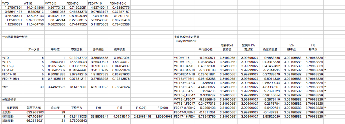
Student's T testはexcelでも特に難しくない。標準関数でできるからね。それに比べて多重検定はアドインとか手計算とか結構面倒なので、これをwebアプリでチョチョイとできるとすごくいい。というわけでまずはexcelで実施した場合。
https://www.amazon.co.jp/dp/4434211625/ref=cm_sw_em_r_mt_dp_U_y7YcEb6ERHBNK

- 作者:柳井久江
- 発売日: 2015/10/20
- メディア: 単行本
この本(正確にはこの第3版)の付録のアドインで解析した結果。
検定統計量の絶対値が水準点より大きいと有意差があると判定される(アスタリスクのついているところ)。
さてこういうのをpythonで行うにはstatsmodels.stats.multicompモジュールの pairwise_tukeyhsd (Tukey's Honest Significant Difference)関数を用いるらしい。
$ python3
Python 3.6.5 (default, Apr 25 2018, 14:26:36)
[GCC 4.2.1 Compatible Apple LLVM 9.0.0 (clang-900.0.39.2)] on darwin
Type "help", "copyright", "credits" or "license" for more information.
>>> from statsmodels.stats.multicomp import pairwise_tukeyhsd
>>> import numpy as np
>>> A = np.array([1.375679545,0.686414272,0.557466114,1.256839102,1.123600968])
>>> B = np.array([14.04818061,5.350681195,13.82671427,9.978383591,11.54647591])
>>> C = np.array([0.867704526,1.059910525,0.954219068,1.061427443,0.882509883])
>>> D = np.array([0.748020814,0.455333729,0.601030484,0.275500152,0.741495253])
>>> E = np.array([4.937450411,9.076321974,8.039161896,5.332406264,5.118753692])
>>> F = np.array([0.482907748,0.372571868,0.929118102,0.997754185,0.79455389])
>>> data_arr = np.hstack( (A,B,C,D,E,F) )
>>> ind_arr = np.repeat(list('ABCDEF'),len(A))
>>> print(pairwise_tukeyhsd(data_arr,ind_arr))
 Multiple Comparison of Means - Tukey HSD, FWER=0.05
=====================================================
group1 group2 meandiff p-adj   lower    upper  reject
-----------------------------------------------------
     A      B   9.9501  0.001   6.7007 13.1995   True
     A      C  -0.0348    0.9  -3.2843  3.2146  False
     A      D  -0.4357    0.9  -3.6851  2.8137  False
     A      E   5.5008  0.001   2.2514  8.7502   True
     A      F  -0.2846    0.9   -3.534  2.9648  False
     B      C  -9.9849  0.001 -13.2344 -6.7355   True
     B      D -10.3858  0.001 -13.6352 -7.1364   True
     B      E  -4.4493 0.0035  -7.6987 -1.1999   True
     B      F -10.2347  0.001 -13.4841 -6.9853   True
     C      D  -0.4009    0.9  -3.6503  2.8485  False
     C      E   5.5357  0.001   2.2862  8.7851   True
     C      F  -0.2498    0.9  -3.4992  2.9996  False
     D      E   5.9365  0.001   2.6871   9.186   True
     D      F   0.1511    0.9  -3.0983  3.4005  False
     E      F  -5.7854  0.001  -9.0349  -2.536   True
-----------------------------------------------------ほうほう、それっぽい結果になった。5%水準で、2つの間に差がないという仮説が棄却されるとTrueなので、上のexcelの結果と完全に一致したと言える。1%水準でどうなるのかはどういうオプションを付けるのだろうか?
あと、アプリ化するにはどういう方向で設計しようか。
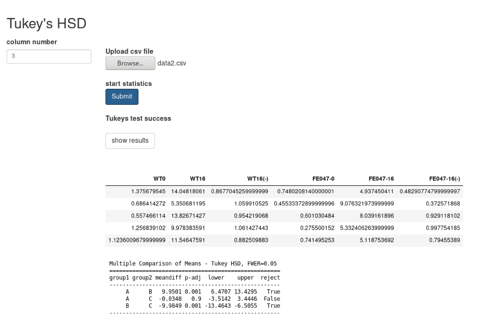
比較する項目数をどう処理しようか考え中。
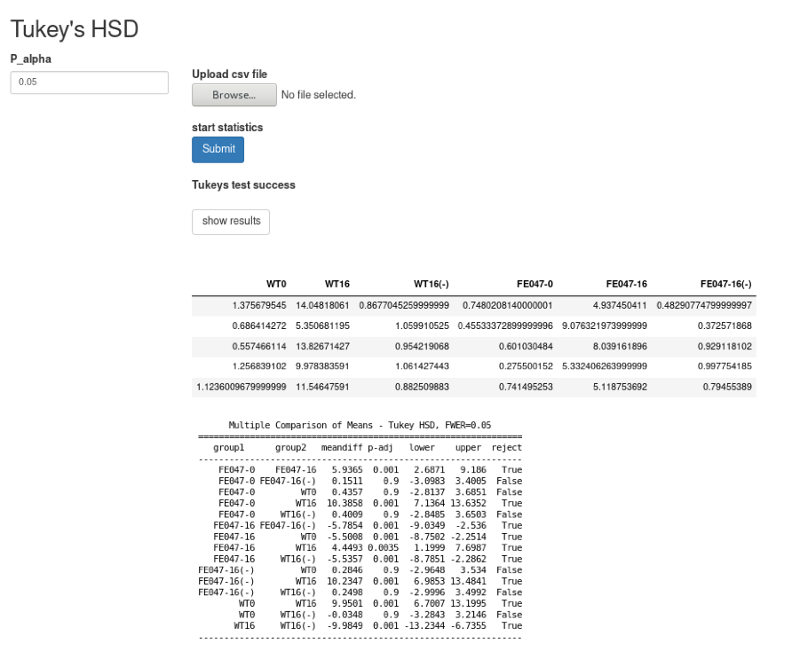
for ループで回すとよいのだろうけど、ちょっと泥臭くif分岐でごまかした。多重比較と言っても12以上も比較することはないだろうからよかろう。
@app.route('/tukey', methods=['GET', 'POST'])
def tukey_index():
    user = g.user.name
    form=StatForm()
    dir = "./user/" + user + "/tukey"
    if os.path.exists(dir):
        shutil.rmtree(dir)
    if not os.path.exists(dir):
        os.makedirs(dir)
    input = dir + "/input.txt"
    output = dir + "/results.txt"

    if request.method == 'POST':
        if 'file' not in request.files:
            flash('No file part')
            return redirect(request.url)
        file = request.files['file']
        if file.filename == '':
            flash('No selected file')
            return redirect(request.url)
        if file and allowed_file(file.filename):
            file.save(input)

        # if form.col1.data:
        #     col1 = form.col1
        # if form.col2.data:
        #     col2 = form.col2
        df = pd.read_csv(input)
        header = df.columns
        record = df.values.tolist()

        # dfs1 = df.iloc[:, 0]
        # dfs2 = df.iloc[:, 1]
        # dfs3 = df.iloc[:, 2]
        data_0 = np.array(df.iloc[:, 0].values.tolist())
        data_1 = np.array(df.iloc[:, 1].values.tolist())
        data_2 = np.array(df.iloc[:, 2].values.tolist())

        # if form.n_samp.data == 3:
        data_arr = np.hstack((data_0,data_1,data_2))
        # ind_arr = np.repeat(list('abc'),len(data_0))
        ind_arr = np.array([])
        ind_arr = np.append(ind_arr, np.repeat(header[0],len(data_0)))
        ind_arr = np.append(ind_arr, np.repeat(header[1],len(data_1)))
        ind_arr = np.append(ind_arr, np.repeat(header[2],len(data_2)))

        count = len(header)-3
        if count > 0:
            count = count -1
            data_3 = np.array(df.iloc[:, 3].values.tolist())
            data_arr = np.hstack((data_0,data_1,data_2,data_3))
            ind_arr = np.append(ind_arr, np.repeat(header[3],len(data_3)))
            if count > 0:
                count = count -1
                data_4 = np.array(df.iloc[:, 4].values.tolist())
                data_arr = np.hstack((data_0,data_1,data_2,data_3,data_4))
                ind_arr = np.append(ind_arr, np.repeat(header[4],len(data_4)))
                if count > 0:
                    count = count -1
                    data_5 = np.array(df.iloc[:, 5].values.tolist())
                    data_arr = np.hstack((data_0,data_1,data_2,data_3,data_4,data_5))
                    ind_arr = np.append(ind_arr, np.repeat(header[5],len(data_5)))
                    if count > 0:
                        count = count -1
                        data_5 = np.array(df.iloc[:, 6].values.tolist())
                        data_arr = np.hstack((data_0,data_1,data_2,data_3,data_4,data_5,data_6))
                        ind_arr = np.append(ind_arr, np.repeat(header[6],len(data_6)))
                        if count > 0:
                            count = count -1
                            data_5 = np.array(df.iloc[:, 7].values.tolist())
                            data_arr = np.hstack((data_0,data_1,data_2,data_3,data_4,data_5,data_6,data_7))
                            ind_arr = np.append(ind_arr, np.repeat(header[7],len(data_7)))
                            if count > 0:
                                count = count -1
                                data_5 = np.array(df.iloc[:, 8].values.tolist())
                                data_arr = np.hstack((data_0,data_1,data_2,data_3,data_4,data_5,data_6,data_7,data_8))
                                ind_arr = np.append(ind_arr, np.repeat(header[8],len(data_8)))
                                if count > 0:
                                    count = count -1
                                    data_5 = np.array(df.iloc[:, 9].values.tolist())
                                    data_arr = np.hstack((data_0,data_1,data_2,data_3,data_4,data_5,data_6,data_7,data_8,data_9))
                                    ind_arr = np.append(ind_arr, np.repeat(header[9],len(data_9)))
                                    if count > 0:
                                        count = count -1
                                        data_5 = np.array(df.iloc[:, 10].values.tolist())
                                        data_arr = np.hstack((data_0,data_1,data_2,data_3,data_4,data_5,data_6,data_7,data_8,data_9,data_10))
                                        ind_arr = np.append(ind_arr, np.repeat(header[10],len(data_10)))
                                        if count > 0:
                                            count = count -1
                                            data_5 = np.array(df.iloc[:, 11].values.tolist())
                                            data_arr = np.hstack((data_0,data_1,data_2,data_3,data_4,data_5,data_6,data_7,data_8,data_9,data_10,data_11))
                                            ind_arr = np.append(ind_arr, np.repeat(header[11],len(data_11)))

        results = str(pairwise_tukeyhsd(data_arr,ind_arr, alpha=form.alpha.data))
        with open(output, mode='w') as f:
            f.write(results)
        link='Tukeys test success<br><br><a href="/tukey/dl/" target="info2" class="btn btn-default">show results</a>'
        return render_template('/tools/tukey.html', form=form, link=link, header=header, record=record)

    return render_template('/tools/tukey.html', form=form)

@app.route('/tukey/dl/')
def dl_tukey_index():
    user = g.user.name
    dir = "./user/" + user + "/tukey"
    if os.path.exists(dir):
        result = dir +"/results.txt"
        f = open(result, 'r')
        return Response(f.read(), mimetype='text/plain')
統計的検定をpythonで行う〜Student's T test編
統計計算をexcel以外でやる。よく使われるのはRなんだがRはいまいち知らないので、pythonでやれないものかと。まあやれるでしょう。いつものようによく使う機能はまとめてWEBアプリにしてやろう。

このグラフデータについてexcelとpythonの比較をしてみる。

AのJA 20 μMのT検定結果はp value = 0.015736074となっている。
これをpythonでやてみる。
$ python3
Python 3.6.5 (default, Apr 25 2018, 14:26:36)
[GCC 4.2.1 Compatible Apple LLVM 9.0.0 (clang-900.0.39.2)] on darwin
Type "help", "copyright", "credits" or "license" for more information.
>>> import numpy as np
>>> from scipy import stats
>>> a = np.array([12,11,12,10,8])
>>> b = np.array([19,14,19,16,11])
>>> stats.ttest_ind(a,b,equal_var = True)
Ttest_indResult(statistic=-3.0535451414764587, pvalue=0.01573607368058338)
このようにちゃんと一致する。
なお等分散性を仮定(equal_var = True)している。

一応アプリにしたけど愛想なさすぎる?

一応これでよさげ。
参考ページ
pandasでcsv/tsvファイル読み込み(read_csv, read_table) | note.nkmk.me
PCA plotをpythonで行うWEBアプリ(ver2)
さて、さっきのアプリからPCAだけを抜き出してちょっと改変してみる。
主成分分析を Python で理解する - Qiita
こちらのページを参考にさせてもらう。
ポイントはnumpyで数値データを抜き出していた点をpandasに換えることでテキストも含んだcsvを入り口にできるようにした点とクラスわけを色で塗り分けるようにした点。
おまけでfigure sizeを設定できるようにもしてみた。
前に作ったstat.pyに以下の記述を追加した。
@app.route('/stat2', methods=['GET', 'POST'])
def stat2_index():
    user = g.user.name
    form=StatForm()
    dir = "./user/" + user + "/stat"
    if os.path.exists(dir):
        shutil.rmtree(dir)
    if not os.path.exists(dir):
        os.makedirs(dir)
    input = dir + "/input.txt"
    output = dir + "/output.txt"


    if request.method == 'POST':
        if 'file' not in request.files:
            flash('No file part')
            return redirect(request.url)
        file = request.files['file']
        if file.filename == '':
            flash('No selected file')
            return redirect(request.url)
        if file and allowed_file(file.filename):
            file.save(input)

        stat_fig = dir + "/stat_" + str(time.time()) + ".png"
        if form.fig_x.data:
        	fig_x=form.fig_x.data
        if form.fig_y.data:
        	fig_y=form.fig_y.data

        df = pd.read_csv(input, sep=",", index_col=0)
        dfs = df.iloc[:, 1:].apply(lambda x: (x-x.mean())/x.std(), axis=0)
        pca = PCA()
        feature = pca.fit(dfs)
        feature = pca.transform(dfs)
        plt.figure(figsize=(fig_x,fig_y))
        plt.scatter(feature[:, 0], feature[:, 1], alpha=0.8, c=list(df.iloc[:, 0]))
        plt.grid()
        plt.title('principal component')
        plt.xlabel("PC1")
        plt.ylabel("PC2")
        plt.savefig(stat_fig)
        img_url = "../../static/" + stat_fig
        return render_template('/tools/stat2.html', form=form, img_url=img_url)

    return render_template('/tools/stat2.html', form=form)
templateの方は殆ど変わらないが
stat2.html
{% extends "base.html" %}
{% import "bootstrap/wtf.html" as wtf %}

{% block title %}Statistics_tool{% endblock %}

{% block head %}
{{ super() }}


{% endblock %}

{% block scripts %}
{{ super() }}
{% endblock %}

{% block page_top %}
<h2>PCA tool</h2>
<div class="row">
  <form class="form form-group form-group-sm" method=post enctype=multipart/form-data>
  <div class="col-xs-2">
    <h4>Figure setting</h4>
    <h5>
    figure_x size  <br>
    {{ form.fig_x }}<br><br>
    figure_y size <br>
    {{ form.fig_y }}<br><br>
      </h5>
  </div>

  <div class="col-xs-10">

    <br>
      <b>Upload csv file</b><br>
      <input type=file name=file>
<br>
      <b>start statistics</b><br>

      <input class='btn btn-primary' type=submit value=Submit>

    {% if img_url %}
    <p><img src="{{ img_url }}"></p>
      {% endif %}
      <br><br>

    {% for message in get_flashed_messages() %}
        <div class="alert alert-success">{{ message }}</div>
        {% endfor %}
    <br><br>
    <div>
    <iframe name="info2" frameborder="0" width=1220px height=600px></iframe>
    </div>
  </div>
    </form>
</div>

{% endblock %}

{% block left %}
{% endblock %}

{% block right %}
{% endblock %}

{% block page_bottom %}

{% endblock %}

要素の側のプロットもつけられるようにした。これでほぼ完成。
PCAやMDS plotをpythonで行うWEBアプリ(ver1)
以前にもpythonでPCAを実施するスクリプトを書いてみていたが、webアプリ版を作ってみた。まずは低機能にとりあえず数値だけのcsvファイルを投げるとプロットを描かせるだけのものから
こんな感じ。
Flaskのviewsはこんなふうで。
/flask_root_folder/app/views/stat.py
# PCA, MDS, tSNEのプロットを作成する
from functools import wraps
from flask import request, redirect, url_for, render_template, flash, Blueprint, session, g, send_file, current_app, Response
from flask_wtf import FlaskForm
from wtforms import SubmitField, SelectField
from werkzeug.utils import secure_filename
import csv, os, shutil, subprocess, sys, re, time
import numpy as np
from matplotlib import pyplot as plt
from sklearn.decomposition import PCA
from sklearn.manifold import MDS, TSNE
import matplotlib
import matplotlib.pyplot as plt

app = Blueprint('stat', __name__)
ALLOWED_EXTENSIONS = set(['txt', 'csv'])   #選択できる入力ファイルの拡張子
def allowed_file(filename):
    return '.' in filename and filename.rsplit('.', 1)[1].lower() in ALLOWED_EXTENSIONS

class StatForm(FlaskForm):
    stat_type = SelectField('statistics type', choices=[('PCA', 'PCA'), ('MDS', 'MDS'), ('tSNE', 'tSNE')])
    submit = SubmitField('Submit')

@app.route('/stat', methods=['GET', 'POST'])
def stat_index():
    user = g.user.name
    form=StatForm()
    dir = "./user/" + user + "/stat"
    if os.path.exists(dir):
        shutil.rmtree(dir)
    if not os.path.exists(dir):
        os.makedirs(dir)
    input = dir + "/input.txt"
    output = dir + "/output.txt"

#ファイルをアップロードして入力する
    if request.method == 'POST':
        if 'file' not in request.files:
            flash('No file part')
            return redirect(request.url) #ファイルが許可された形式でないとエラーを返す
        file = request.files['file']
        if file.filename == '':
            flash('No selected file')
            return redirect(request.url) #ファイルが選択されていないとエラーを返す
        if file and allowed_file(file.filename):
            file.save(input) #ファイルをinputに保存する
        npArray = np.loadtxt(input, delimiter = ",")
        X = np.array(npArray)
        stat_fig = dir + "/stat_" + str(time.time()) + ".png"

        if form.stat_type.data == "PCA":

            pca = PCA()
            pca.fit(X)
            transformed = pca.fit_transform(X)
            plt.figure()
            plt.scatter(transformed[:, 0], transformed[:, 1])
            plt.title('principal component')
            plt.xlabel('pc1')
            plt.ylabel('pc2')
            stat_result = pca.explained_variance_ratio_
            plt.savefig(stat_fig)
            img_url = "../../static/" + stat_fig # flask_root_folder/app/staticにflask_root_folder/userのリンクを張ってある

            return render_template('/tools/stat.html', stat_result=stat_result, form=form, img_url=img_url)

        if form.stat_type.data == "MDS":

            mds = MDS(n_jobs=4)
            mds.fit(X)
            transformed = mds.fit_transform(X)
            plt.figure()
            plt.scatter(transformed[:, 0], transformed[:, 1])
            plt.title('Multidimensional scaling')
            plt.savefig(stat_fig)
            img_url = "../../static/" + stat_fig

            return render_template('/tools/stat.html', form=form, img_url=img_url)

        if form.stat_type.data == "tSNE":

            tsne = TSNE()
            tsne.fit(X)
            transformed = tsne.fit_transform(X)
            plt.figure()
            plt.scatter(transformed[:, 0], transformed[:, 1])
            plt.title('t-distributed Stochastic Neighbor embedding')
            plt.savefig(stat_fig)
            img_url = "../../static/" + stat_fig

            return render_template('/tools/stat.html', form=form, img_url=img_url)

    return render_template('/tools/stat.html', form=form)
template
flask_root_folder/app/templates/tools/stat.html
{% extends "base.html" %}
{% import "bootstrap/wtf.html" as wtf %}

{% block title %}Statistics_tool{% endblock %}

{% block head %}
{{ super() }}


{% endblock %}

{% block scripts %}
{{ super() }}
{% endblock %}

{% block page_top %}
<h2>Statistics tool</h2>
<div class="row">
  <form class="form form-group form-group-sm" method=post enctype=multipart/form-data>
  <div class="col-xs-1">
  </div>

  <div class="col-xs-10">

    <br>
      <b>Upload csv file</b><br>
      <input type=file name=file>
<br>
      <b>statistics type</b><br>
      {{ form.stat_type }}<br><br>
      <b>start statistics</b><br>

      <input class='btn btn-primary' type=submit value=Submit>


    {% if img_url %}
    <p><img src="{{ img_url }}"></p>
      {% endif %}
      <br><br>
      {{ stat_result|safe }}<br>
    {% for message in get_flashed_messages() %}
        <div class="alert alert-success">{{ message }}</div>
        {% endfor %}
    <br><br>

  </div>
    </form>
</div>
<div class="col-xs-1">
</div>
{% endblock %}

{% block left %}
{% endblock %}

{% block right %}
{% endblock %}

{% block page_bottom %}

{% endblock %}
firewall-cmdのお作法
これまたしょっちゅう・・・
activeなゾーンの表示
# firewall-cmd --list-all
public (active)
  target: default
  icmp-block-inversion: no
  interfaces: eth0
  sources:
  services: dhcpv6-client ssh
  ports:
  protocols:
  masquerade: no
  forward-ports:
  source-ports:
  icmp-blocks:
  rich rules:
似ているけど
# firewall-cmd --list-all-zones
block
  target: %%REJECT%%
  icmp-block-inversion: no
  interfaces:
  sources:
  services:
  ports:
  protocols:
  masquerade: no
  forward-ports:
  source-ports:
  icmp-blocks:
  rich rules:


dmz
  target: default
  icmp-block-inversion: no
  interfaces:
  sources:
  services: ssh
  ports:
  protocols:
  masquerade: no
  forward-ports:
  source-ports:
  icmp-blocks:
  rich rules:

・・・・・・

work
  target: default
  icmp-block-inversion: no
  interfaces:
  sources:
  services: dhcpv6-client ssh
  ports:
  protocols:
  masquerade: no
  forward-ports:
  source-ports:
  icmp-blocks:
  rich rules:
こんな感じにずらずらと一覧。
get系
# firewall-cmd --get-active-zones
public
  interfaces: eth0

# firewall-cmd --get-default-zone
public

# firewall-cmd --get-services
RH-Satellite-6 amanda-client amanda-k5-client amqp amqps apcupsd audit bacula bacula-client bgp bitcoin bitcoin-rpc bitcoin-testnet bitcoin-testnet-rpc ceph ceph-mon cfengine condor-collector ctdb dhcp dhcpv6 dhcpv6-client distcc dns docker-registry docker-swarm dropbox-lansync elasticsearch etcd-client etcd-server finger freeipa-ldap freeipa-ldaps freeipa-replication freeipa-trust ftp ganglia-client ganglia-master git gre high-availability http https imap imaps ipp ipp-client ipsec irc ircs iscsi-target isns jenkins kadmin kerberos kibana klogin kpasswd kprop kshell ldap ldaps libvirt libvirt-tls lightning-network llmnr managesieve matrix mdns minidlna mongodb mosh mountd mqtt mqtt-tls ms-wbt mssql murmur mysql nfs nfs3 nmea-0183 nrpe ntp nut openvpn ovirt-imageio ovirt-storageconsole ovirt-vmconsole plex pmcd pmproxy pmwebapi pmwebapis pop3 pop3s postgresql privoxy proxy-dhcp ptp pulseaudio puppetmaster quassel radius redis rpc-bind rsh rsyncd rtsp salt-master samba samba-client samba-dc sane sip sips slp smtp smtp-submission smtps snmp snmptrap spideroak-lansync squid ssh steam-streaming svdrp svn syncthing syncthing-gui synergy syslog syslog-tls telnet tftp tftp-client tinc tor-socks transmission-client upnp-client vdsm vnc-server wbem-http wbem-https wsman wsmans xdmcp xmpp-bosh xmpp-client xmpp-local xmpp-server zabbix-agent zabbix-server
serviceは
/usr/lib/firewalld/services/
にxmlファイルとして定義されているもの
# firewall-cmd --add-service=https --zone=public --permanent
# firewall-cmd --reload
success
というふうに開通したいサービスをゾーンに登録できる
permanentオプションをつけると起動時に自動で開き、つけないとその時限りとなる。permanentオプションを付けるときはreloadオプションも必要。
# firewall-cmd --add-port=8080/tcp --zone=public
ポートを直接指定して開く場合はこのようにする。通常のサービスとは異なるポートを使いたいときなど。
nmcliのお作法
すぐに忘れてしょっちゅう調べている気がするので、覚書。
基本のネットワーク設定
# nmcli c m eth0 ipv4.method manual ipv4.addresses 192.168.1.101/24 ipv4.gateway 192.168.1.1 ipv4.dns 8.8.8.8 connection.autoconnect yes
この例ではDHCPをやめて手動設定にする、ipアドレス、ゲートウェイアドレス、DNSサーバ、そして起動時に自動でネットワークデバイスを有効にする設定を一気に行っているが、必要な部分だけを書いてもいい。
設定変更したあとは再起動するか、
# nmcli c down eth0; nmcli c up eth0
でネットワークをリセットする。
現在の状況を表示
# nmcli d
DEVICE  TYPE      STATE      CONNECTION
eth0    ethernet  connected  eth0
lo      loopback  unmanaged  --
firewalldで使うゾーンの設定も行える。
# nmcli c m eth0 connection.zone internal
なお、nmcli c のcはconnectionの省略でcと書く代わりにconnectionと書いてもいい。
  g[eneral]       NetworkManager's general status and operations
  n[etworking]    overall networking control
  r[adio]         NetworkManager radio switches
  c[onnection]    NetworkManager's connections
  d[evice]        devices managed by NetworkManager
  a[gent]         NetworkManager secret agent or polkit agent
  m[onitor]       monitor NetworkManager changes
またnmcli c mのmはmodifyの省略形でmodやmodifyでもいいようだ。